To view the presentation, please click on the below link:
http://www.slideshare.net/minh65/electrocardiogram-ecg-or-ekg
Saturday, August 27, 2016
Sunday, August 21, 2016
To view the presentation, please click the below link:
http://www.slideshare.net/minh65/simulation-results-of-induction-heating-coil
http://www.slideshare.net/minh65/simulation-results-of-induction-heating-coil
Friday, August 19, 2016
matlab code to study upsampling(Sampling rate) of audio file
%% matlab code to study upsampling(Sampling rate) of audio file
% sounds like a problem of asynchronous sample rate conversion.
% To convert from one sample rate to another:
% use sinc interpolation to compute the continuous time representation
% of the signal then resample at our new sample rate.
% resample the signal to have sample times that are fixed.
% Read in the sound
% returns the sample rate(FS) in Hertz
% N = number sample
% the number of bits per sample (BITS) used to encode the data in the file
% Minh Anh Nguyen
% minhanhnguyen@q.com
% close
close all; % Close all figures (except those of imtool.)
clear; % Erase all existing variables.
clc;% Clear the command window.
imtool close all; % Close all imtool figures.
workspace; % Make sure the workspace panel is showing.
%% read and plot .wav file
figure;
myvoice1 = audioread('good2.wav');
% Reads in the sound file, into a big array called y.
[y1, fs1] = audioread('good2.wav');
size(y1);
left1=y1(:,1);
right1=y1(:,2);
N = length(right1);
% Normalize y; that is, scale all values to its maximum.
y = right1/max(abs(right1));
t1 = (0:1:N-1)/fs1;
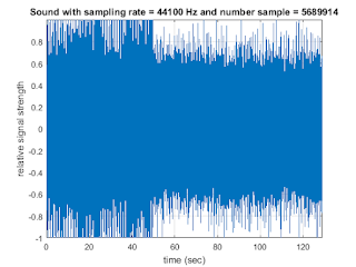
plot(t1,right1 );
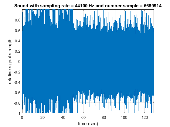
str1=sprintf('Sound with sampling rate = %d Hz and number sample = %d', fs1, N);
title(str1);
xlabel('time (sec)'); ylabel('relative signal strength'); grid on;
axis tight
grid on;
%% Compute the power spectral density, a measurement of the energy at various frequencies
% DFT to describe the signal in the frequency
NFFT = 2 ^ nextpow2(N);
Y = fft(y1, NFFT) / N;
f = (fs1 / 2 * linspace(0, 1, NFFT / 2+1))'; % Vector containing frequencies in Hz
amp = ( 2 * abs(Y(1: NFFT / 2+1))); % Vector containing corresponding amplitudes
figure;
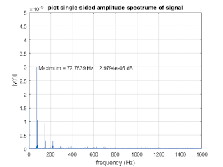
plot (f, amp); xlim([0,1600]); ylim([0,0.5e-4]);
title ('plot single-sided amplitude spectrume of signal')
xlabel ('frequency (Hz)')
ylabel ('|y(f)|')
grid on;
% display markers at specific data points on DFT graph
indexmin1 = find(min(amp) == amp);
xmin1 = f(indexmin1);
ymin1 = amp(indexmin1);
indexmax1 = find(max(amp) == amp);
xmax1 = f(indexmax1);
ymax1 = amp(indexmax1);
strmax1 = [' Maximum = ',num2str(xmax1),' Hz',' ', num2str(ymax1),' dB'];
text(xmax1,ymax1,strmax1,'HorizontalAlignment','Left');
fsorg=44100;
fs = 8000;
%% resample is your function. To downsample signal from 44100 Hz to 8000 Hz:
%(the "1" and "2" arguments define the resampling ratio: 8000/44100 = 1/2)
%To upsample back to 44100 Hz: x2 = resample(y,2,1);
figure;
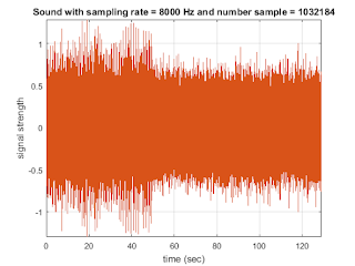
y_1 = resample(y1,fs,fsorg);
N1_1 = length(y_1);
t1_1 = (0:1:length(y_1)-1)/fs;
plot(t1_1, y_1);
str1=sprintf('Sound with sampling rate = %d Hz and number sample = %d', fs, N1_1);
title(str1);
xlabel('time (sec)');
ylabel('signal strength')
axis tight
grid;
%% Compute the power spectral density, a measurement of the energy at various frequencies
% DFT to describe the signal in the frequency
NFFTd = 2 ^ nextpow2(N1_1);
Yd = fft(y_1, NFFTd) / N1_1;
fd = (fs / 2 * linspace(0, 1, NFFTd / 2+1))'; % Vector containing frequencies in Hz
amp_down = ( 2 * abs(Yd(1: NFFTd / 2+1))); % Vector containing corresponding amplitudes
figure;
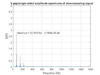
plot (fd, amp_down); xlim([0,1600]); ylim([0,0.5e-4]);
title ('\t plot single-sided amplitude spectrume of downsampling signal')
xlabel ('frequency (Hz)')
ylabel ('|y(f)|')
grid on;
% display markers at specific data points on DFT graph
indexmin1 = find(min(amp_down) == amp_down);
xmin1 = fd(indexmin1);
ymin1 = amp_down(indexmin1);
indexmax1 = find(max(amp_down) == amp_down);
xmax1 = fd(indexmax1);
ymax1 = amp_down(indexmax1);
strmax1 = [' Maximum = ',num2str(xmax1),' Hz',' ', num2str(ymax1),' dB'];
text(xmax1,ymax1,strmax1,'HorizontalAlignment','Left');
% sounds like a problem of asynchronous sample rate conversion.
% To convert from one sample rate to another:
% use sinc interpolation to compute the continuous time representation
% of the signal then resample at our new sample rate.
% resample the signal to have sample times that are fixed.
% Read in the sound
% returns the sample rate(FS) in Hertz
% N = number sample
% the number of bits per sample (BITS) used to encode the data in the file
% Minh Anh Nguyen
% minhanhnguyen@q.com
% close
close all; % Close all figures (except those of imtool.)
clear; % Erase all existing variables.
clc;% Clear the command window.
imtool close all; % Close all imtool figures.
workspace; % Make sure the workspace panel is showing.
%% read and plot .wav file
figure;
myvoice1 = audioread('good2.wav');
% Reads in the sound file, into a big array called y.
[y1, fs1] = audioread('good2.wav');
size(y1);
left1=y1(:,1);
right1=y1(:,2);
N = length(right1);
% Normalize y; that is, scale all values to its maximum.
y = right1/max(abs(right1));
t1 = (0:1:N-1)/fs1;
plot(t1,right1 );
str1=sprintf('Sound with sampling rate = %d Hz and number sample = %d', fs1, N);
title(str1);
xlabel('time (sec)'); ylabel('relative signal strength'); grid on;
axis tight
grid on;
%% Compute the power spectral density, a measurement of the energy at various frequencies
% DFT to describe the signal in the frequency
NFFT = 2 ^ nextpow2(N);
Y = fft(y1, NFFT) / N;
f = (fs1 / 2 * linspace(0, 1, NFFT / 2+1))'; % Vector containing frequencies in Hz
amp = ( 2 * abs(Y(1: NFFT / 2+1))); % Vector containing corresponding amplitudes
figure;
plot (f, amp); xlim([0,1600]); ylim([0,0.5e-4]);
title ('plot single-sided amplitude spectrume of signal')
xlabel ('frequency (Hz)')
ylabel ('|y(f)|')
grid on;
% display markers at specific data points on DFT graph
indexmin1 = find(min(amp) == amp);
xmin1 = f(indexmin1);
ymin1 = amp(indexmin1);
indexmax1 = find(max(amp) == amp);
xmax1 = f(indexmax1);
ymax1 = amp(indexmax1);
strmax1 = [' Maximum = ',num2str(xmax1),' Hz',' ', num2str(ymax1),' dB'];
text(xmax1,ymax1,strmax1,'HorizontalAlignment','Left');

fsorg=44100;
fs = 8000;
%% resample is your function. To downsample signal from 44100 Hz to 8000 Hz:
%(the "1" and "2" arguments define the resampling ratio: 8000/44100 = 1/2)
%To upsample back to 44100 Hz: x2 = resample(y,2,1);
figure;
y_1 = resample(y1,fs,fsorg);
N1_1 = length(y_1);
t1_1 = (0:1:length(y_1)-1)/fs;
plot(t1_1, y_1);
str1=sprintf('Sound with sampling rate = %d Hz and number sample = %d', fs, N1_1);
title(str1);
xlabel('time (sec)');
ylabel('signal strength')
axis tight
grid;

%% Compute the power spectral density, a measurement of the energy at various frequencies
% DFT to describe the signal in the frequency
NFFTd = 2 ^ nextpow2(N1_1);
Yd = fft(y_1, NFFTd) / N1_1;
fd = (fs / 2 * linspace(0, 1, NFFTd / 2+1))'; % Vector containing frequencies in Hz
amp_down = ( 2 * abs(Yd(1: NFFTd / 2+1))); % Vector containing corresponding amplitudes
figure;
plot (fd, amp_down); xlim([0,1600]); ylim([0,0.5e-4]);
title ('\t plot single-sided amplitude spectrume of downsampling signal')
xlabel ('frequency (Hz)')
ylabel ('|y(f)|')
grid on;
% display markers at specific data points on DFT graph
indexmin1 = find(min(amp_down) == amp_down);
xmin1 = fd(indexmin1);
ymin1 = amp_down(indexmin1);
indexmax1 = find(max(amp_down) == amp_down);
xmax1 = fd(indexmax1);
ymax1 = amp_down(indexmax1);
strmax1 = [' Maximum = ',num2str(xmax1),' Hz',' ', num2str(ymax1),' dB'];
text(xmax1,ymax1,strmax1,'HorizontalAlignment','Left');

Matlab code to compute the corresponding absorption coefficients
%% oxyhemoglobin and deoxyhemoglobin extinction.m
% Author:Minh Anh Nguyen
% minhanhnguyen@q.com
% Matlab code to compute the corresponding absorption coefficients and plot
% the three absorption spectra on the same graph.
% Identify the low-absorption near-IR window that provide deep
% penetration.
% data for molar extinction coefficients of oxy-and deoxyhemoglobin and
% absorption coefficient of pure water as a function of wavelength are
% copied directly from this website: http://omlc.org/spectra/hemoglobin/summary.html
% Use physiologically representative values for both oxygen saturation SO2
% and total concentration of hemoglobin CHb.
% These values for the molar extinction coefficient e in [cm-1/(moles/liter)] were compiled by Scott Prahl using data from
%W. B. Gratzer, Med. Res. Council Labs, Holly Hill, London
%N. Kollias, Wellman Laboratories, Harvard Medical School, Boston
%To convert this data to absorbance A, multiply by the molar concentration and the pathlength. For example, if x is the number of grams per liter and a 1 cm cuvette is being used, then the absorbance is given by
%(e) [(1/cm)/(moles/liter)] (x) [g/liter] (1) [cm]
%A = ---------------------------------------------------
% 64,500 [g/mole]
%using 64,500 as the gram molecular weight of hemoglobin.
%To convert this data to absorption coefficient in (cm-1), multiply by the molar concentration and 2.303,
% µa = (2.303) e (x g/liter)/(64,500 g Hb/mole)
%where x is the number of grams per liter. A typical value of x for whole blood is x=150 g Hb/liter.
close all; clear; clc;
load ('oxy_deoxy.mat');
figure;
semilogy(oxy_deoxy(:,1), oxy_deoxy(:,2), 'b', 'linewidth',1.5);
hold on
semilogy(oxy_deoxy(:,1), oxy_deoxy(:,3), 'r', 'linewidth',1.5);
title('The molar oxyhemoglobin and deoxyhemoglobin extinction','FontSize',14);
set(gca,'FontSize',14);
ylabel('molar extinction coefficient (cm^{-1}(moles/l)^{-1})','fontsize',14);
xlabel('wavelength (nm)','fontsize',14);
axis([250 1000 0 10^6]);
set(gcf,'PaperUnits','inches','PaperPosition',[0 0 6 5]);
grid on;
legend('y = HbO2 ','y = Hb')

%% purewater
load ('purewater.mat');
figure;
semilogy(water(:,1), water(:,2), 'b', 'linewidth',1.5);
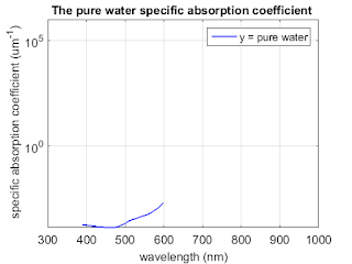
title('The pure water specific absorption coefficient ','FontSize',14);
set(gca,'FontSize',14);
ylabel(' specific absorption coefficient (um^{-1})','fontsize',14);
xlabel('wavelength (nm)','fontsize',14);
axis([300 1000 0 1*10^6]);
set(gcf,'PaperUnits','inches','PaperPosition',[0 0 6 5]);
grid on;
legend('y = pure water')
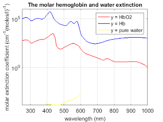
%% all three graph
figure;
semilogy(oxy_deoxy(:,1), oxy_deoxy(:,3)*0.0054, 'r', 'linewidth',1.5);
hold on
semilogy(oxy_deoxy(:,1), oxy_deoxy(:,2), 'b', 'linewidth',1.5);
hold on
semilogy(water(:,1), water(:,2), 'y', 'linewidth',1.5);
title('The molar hemoglobin and water extinction','FontSize',14);
set(gca,'FontSize',14);
ylabel('molar extinction coefficient (cm^{-1}(moles/l)^{-1})','fontsize',14);
xlabel('wavelength (nm)','fontsize',14);
%axis([250 1000 0 0.6*10^6]);
axis([250 1000 0 1*10^6]);
set(gcf,'PaperUnits','inches','PaperPosition',[0 0 6 5]);
grid on;
legend('y = HbO2 ','y = Hb', 'y = pure water')
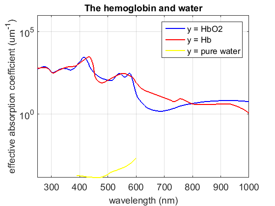
%% Absorption
figure;
semilogy(oxy_deoxy(:,1), oxy_deoxy(:,2)*0.0054, 'b', 'linewidth',1.5);
hold on
semilogy(oxy_deoxy(:,1), oxy_deoxy(:,3)*0.0054, 'r', 'linewidth',1.5);
hold on
semilogy(water(:,1), water(:,2), 'y', 'linewidth',1.5);
title('The hemoglobin and water','FontSize',14);
set(gca,'FontSize',14);
ylabel('effective absorption coefficient (um^{-1})','fontsize',14);
xlabel('wavelength (nm)','fontsize',14);
axis([250 1000 0 1*10^6]);
set(gcf,'PaperUnits','inches','PaperPosition',[0 0 6 5]);
grid on;
legend('y = HbO2 ','y = Hb', 'y = pure water')

% Author:Minh Anh Nguyen
% minhanhnguyen@q.com
% Matlab code to compute the corresponding absorption coefficients and plot
% the three absorption spectra on the same graph.
% Identify the low-absorption near-IR window that provide deep
% penetration.
% data for molar extinction coefficients of oxy-and deoxyhemoglobin and
% absorption coefficient of pure water as a function of wavelength are
% copied directly from this website: http://omlc.org/spectra/hemoglobin/summary.html
% Use physiologically representative values for both oxygen saturation SO2
% and total concentration of hemoglobin CHb.
% These values for the molar extinction coefficient e in [cm-1/(moles/liter)] were compiled by Scott Prahl using data from
%W. B. Gratzer, Med. Res. Council Labs, Holly Hill, London
%N. Kollias, Wellman Laboratories, Harvard Medical School, Boston
%To convert this data to absorbance A, multiply by the molar concentration and the pathlength. For example, if x is the number of grams per liter and a 1 cm cuvette is being used, then the absorbance is given by
%(e) [(1/cm)/(moles/liter)] (x) [g/liter] (1) [cm]
%A = ---------------------------------------------------
% 64,500 [g/mole]
%using 64,500 as the gram molecular weight of hemoglobin.
%To convert this data to absorption coefficient in (cm-1), multiply by the molar concentration and 2.303,
% µa = (2.303) e (x g/liter)/(64,500 g Hb/mole)
%where x is the number of grams per liter. A typical value of x for whole blood is x=150 g Hb/liter.
close all; clear; clc;
load ('oxy_deoxy.mat');
figure;
semilogy(oxy_deoxy(:,1), oxy_deoxy(:,2), 'b', 'linewidth',1.5);
hold on
semilogy(oxy_deoxy(:,1), oxy_deoxy(:,3), 'r', 'linewidth',1.5);
title('The molar oxyhemoglobin and deoxyhemoglobin extinction','FontSize',14);
set(gca,'FontSize',14);
ylabel('molar extinction coefficient (cm^{-1}(moles/l)^{-1})','fontsize',14);
xlabel('wavelength (nm)','fontsize',14);
axis([250 1000 0 10^6]);
set(gcf,'PaperUnits','inches','PaperPosition',[0 0 6 5]);
grid on;
legend('y = HbO2 ','y = Hb')

%% purewater
load ('purewater.mat');
figure;
semilogy(water(:,1), water(:,2), 'b', 'linewidth',1.5);
title('The pure water specific absorption coefficient ','FontSize',14);
set(gca,'FontSize',14);
ylabel(' specific absorption coefficient (um^{-1})','fontsize',14);
xlabel('wavelength (nm)','fontsize',14);
axis([300 1000 0 1*10^6]);
set(gcf,'PaperUnits','inches','PaperPosition',[0 0 6 5]);
grid on;
legend('y = pure water')

%% all three graph
figure;
semilogy(oxy_deoxy(:,1), oxy_deoxy(:,3)*0.0054, 'r', 'linewidth',1.5);
hold on
semilogy(oxy_deoxy(:,1), oxy_deoxy(:,2), 'b', 'linewidth',1.5);
hold on
semilogy(water(:,1), water(:,2), 'y', 'linewidth',1.5);
title('The molar hemoglobin and water extinction','FontSize',14);
set(gca,'FontSize',14);
ylabel('molar extinction coefficient (cm^{-1}(moles/l)^{-1})','fontsize',14);
xlabel('wavelength (nm)','fontsize',14);
%axis([250 1000 0 0.6*10^6]);
axis([250 1000 0 1*10^6]);
set(gcf,'PaperUnits','inches','PaperPosition',[0 0 6 5]);
grid on;
legend('y = HbO2 ','y = Hb', 'y = pure water')

%% Absorption
figure;
semilogy(oxy_deoxy(:,1), oxy_deoxy(:,2)*0.0054, 'b', 'linewidth',1.5);
hold on
semilogy(oxy_deoxy(:,1), oxy_deoxy(:,3)*0.0054, 'r', 'linewidth',1.5);
hold on
semilogy(water(:,1), water(:,2), 'y', 'linewidth',1.5);
title('The hemoglobin and water','FontSize',14);
set(gca,'FontSize',14);
ylabel('effective absorption coefficient (um^{-1})','fontsize',14);
xlabel('wavelength (nm)','fontsize',14);
axis([250 1000 0 1*10^6]);
set(gcf,'PaperUnits','inches','PaperPosition',[0 0 6 5]);
grid on;
legend('y = HbO2 ','y = Hb', 'y = pure water')
Thursday, August 18, 2016
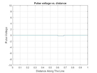
Matlab code to calculate and plot pulses on a lossless transmission line at13.5Mhz
% this matlab code is calculate and plot pulses on a lossless transmission line
% Frequency is 13.5Mhz
%minhanhnguyen@q.com
% Clear the screen
clc;
clear;
% close all windows
close all;
% use these Parameters to calculate and plot Pulse Propagation on a Transline
Ro=50; %Ro = line impedance
Rl=100; %Rl = load resistance
Rg=25; %Rg = generator resistance
Vo=10; %Vo = voltage source
T=.08; %T = pulse width
v=1; %v = wave velocity
d=1; %d = line length
dt=.02; %dt = time step,
n=170; %n = number of time steps
% Voltage Divider at Input
vDivider = (Ro/(Ro+Rg));
% Reflection Coefficient at Load
gamLoad = (Rl-Ro)/(Rl+Ro);
% Reflection Coefficient at Generator
gamGenerator = (Rg-Ro)/(Rg+Ro);
% Transit Time
tTime = d/v;
% Position along the line
x=[0:d/500:d];
for j = 0:n;
% Time
t = j*dt;
% Leading edge of pulse
xl = v*t;
% Trailing edge of pulse
xt = v*(t-T);
% Voltage along the line at time t
V = Vo*(vDivider*(x<xl).*(x>xt));
V = V + Vo*(vDivider*gamLoad)*(x>(2*d-xl)).*(x<(2*d-xt));
V = V + Vo*(vDivider*gamLoad*gamGenerator)*(x<(xl-2*d)).*(x>(xt-2*d));
V = V + Vo*(vDivider*(gamLoad^2)*gamGenerator)*(x>(4*d-xl)).*(x<(4*d-xt));
% Plotting the result
plot(x,V);axis([0 d -Vo Vo]);grid;
title('Pulse voltage vs. distance');
xlabel('Distance Along The Line');
ylabel('Pulse Voltage');
pause(.5)
end
Matlab code to calculate the voltage on the transmission line
% This matlab code is setup for calculating the voltage on the
% transmission line. The code will then plot the results.
% frequency is 13.5Mhz
% Clear the screen
clc;
clear all;
% close all windows
close all;
%% input values
RL = 20; % resistive part of load
CL = 3.3e-9; % capacitive part of load
len = 80; % transmission line length
freq = 13.5e+6; % frequency
omega = 2*pi*freq;
Z0 = 50; % characteristic impedance of line
v = 2e+8; % velocity in RG 58 cable
ZS = 50; % source impedance
%% set up the node measurements with arbitrary values
z_node = [0:4:len]; % equivalent position of nodes on transmission line
V_node = [0 1 2 3.1 4 5 6 7 8.2 9 10 11.4 12 13 14 15 16 17];
V_node = [V_node 18.1 19 20.5];
%%set up phase measurements with arbitrary values
phase_node = [0 1 2 3.1 4 5 6 7 8.2 9 10 11.4 12 13 14 15 16 17];
phase_node = [phase_node 18.1 19 20.5];
%%calculating the transmission line voltage
z = [0:1:len]; % z position on line
ZL = RL - j./omega./CL; % load impedance
V_line = ZL .* z .* exp(-j.*omega.*z./v) ./len;
%% Find the magnitude and angle of the voltage phasor
V_line_mag = abs(V_line);
V_line_deg = 180*angle(V_line)./pi;
%% Plot results
figure(1);
subplot(2,1,1), plot(z,V_line_mag, z_node, V_node, 'o');
title('Unmodified line vs. V magnitude');
ylabel('V magnitude');
legend('trans. line analysis','circuit analysis', 0);
subplot(2,1,2), plot(z,V_line_deg, z_node, phase_node, 'o');
title('Unmodified line vs. phase');
ylabel('phase(degrees)');
xlabel('z position on line (meters)');
legend('trans. line analysis','circuit analysis', 0);
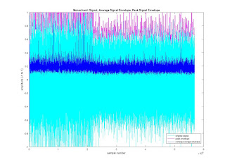
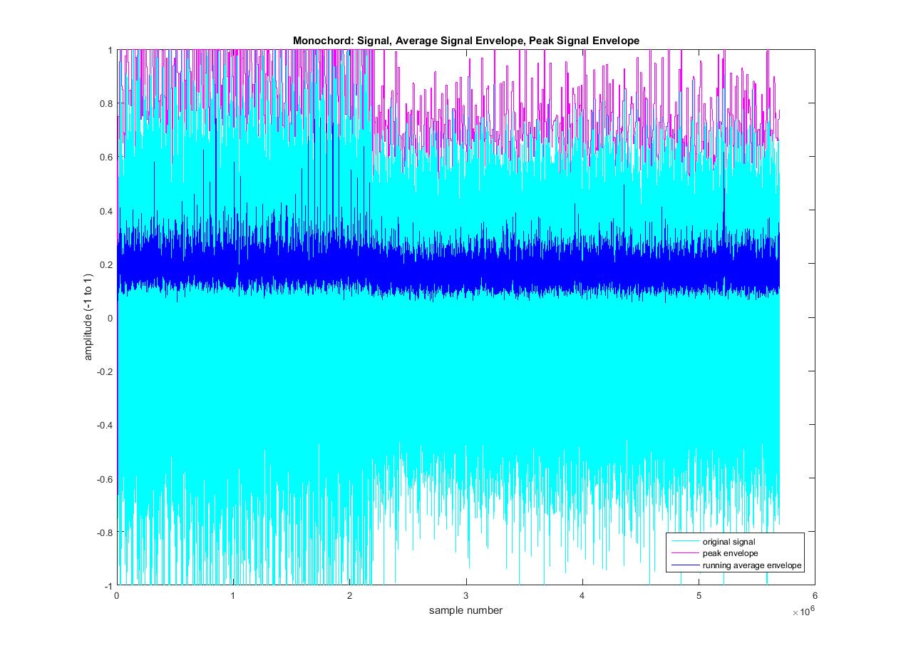
MatLab function to plot Amplitude Envelopes of .wav file
% This MatLab function takes a "wav" sound file as an input
% perform the average and peak envelopes of an input signal,
% and then plot all three plots on a graph.
% usage: amplitude_envelopes ('*.wav')
% Author: Minh Anh Nguyen
% email: minhanhnguyen@q.com
function [amplitude_envelopes] = amplitude_envelopes ( file );
close all;% Close all figures (except those of imtool.)
clf % Clears the graphic screen.
% Reads in the sound file, into a big array called y.
y1=audioread(file);
[y1, fs1]=audioread(file);
size(y1);
left1=y1(:,1);
right1=y1(:,2);
% Normalize y; that is, scale all values to its maximum.
y = right1/max(abs(right1));
% If you want to hear the sound after you read it in
% Sound just plays a file to the speaker.
sound(y, 44100);
% Initialize peak and average arrays to be the same as the signal. We’re
% keeping three big arrays, all of the same length.
average_env = y;
max_env = y;
% Set the window lengths directly, in number of samples.
% the average should be smaller than the peak, since it will tend to
% flatten out if it gets too big.
% average and peak window size are two numbers, which can be played with
% to vary what the pictures will look like.
% Note: use two different window sizes so that we can have
% different kinds of resolution for peak and average charts.
average_window_size = 512;
peak_window_size = 10000;
% from the input signal, taking an average of the previous,
% average window size number of samples, and store that in the current
% place in the average array.
% Use a loop that starts at the end of the first window and goes to the
% end of the sound file, indicated by length(average_env).
% use "sum" command to take some range of a vector.
for k = average_window_size:length(average_env)
running_sum = sum(abs(y(k-average_window_size+1:k)));
average_env(k) = running_sum /average_window_size ;
end
% from the input signal, taking the maximum value of the previous
% peak_window_size number of samples.
for k = peak_window_size:length(max_env)
max_env(k)= max(abs(y(k-peak_window_size+1:k)));
end
% Plot the three "signals": the original in the color cyan, the
% peak in magenta, and the average in blue. The colors are the
% letters in single quotes.
plot(y, 'c')
hold on
plot (max_env, 'm')
hold on
plot(average_env, 'b')
title('Monochord: Signal, Average Signal Envelope, Peak Signal Envelope')
xlabel('sample number')
ylabel('amplitude (-1 to 1)')
legend('original signal', 'peak envelope', 'running average envelope', 0)
Monday, August 15, 2016
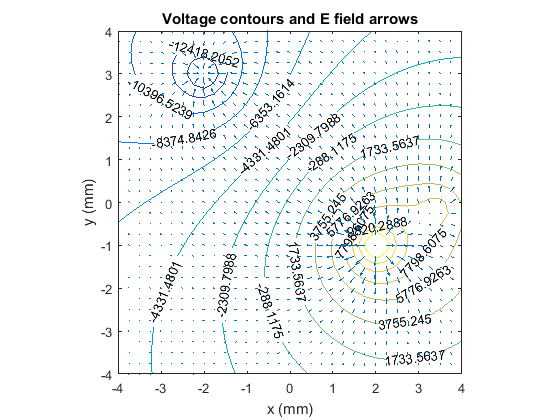
Matlab code to calculate the potential of line charges
Contents
- set up arrays of line charge locations
- strength of each line charge
- plot the Efield arrows and labels for the voltage contours
% Matlab code to calculate the potential due to a set of line charges.  The voltage
% reference is taken as the origin.  The code will have problems if any line
% charges are located at the origin.

% Clear the screen
clc;
clear all;
% close all windows
close all;
set up arrays of line charge locations
xcharge = [3.5 2 -2]; % x position of line charge in mm ycharge = [-0.1 -1 3]; % y position of line charge in mm xcharge = xcharge * .001; % convert to meters ycharge = ycharge * .001;strength of each line charge
rho_l_basic = 1e-7; % units are C/m rho_l = rho_l_basic * [1 3 -2];% Set up grid for plotting Ngrid = 33; gridmax = .004; % grid is the x and y values at which the calculation is done grid = linspace(-gridmax, gridmax, Ngrid); % Calculate voltage on grid due to each charge % create 2 3D grids. size of the arrays are Ngrid x Ngrid x ncharge % The first array represents all combination of xgrid and ygrid % locations with the xposition of the line charge. The second % represents all combinations with the y position of the line charges. [xx1, yy1, xc1] = meshgrid(grid, grid, xcharge); [xx2, yy2, yc2] = meshgrid(grid, grid, ycharge); % Distance between the line charges and the grid points (3D array) dist1 = sqrt( (xx1-xc1).^2 + (yy2 - yc2).^2); % Grid points very close to a line charge will have a very high voltage that % will dominate contour plot. Suppress this. dist1min = .0002; dist1 = max(dist1, dist1min); % distance to reference voltage location (the origin). dist2 = sqrt(xc1.^2 + yc2.^2); % Calculate voltage at each grid point. Vparts is the partial contribution to % the voltage at each grid point (except for a charge strength factor). It is % an(Ngrid x Ngrid x ncharge) array. The loop to calculate Vgrid then sums up % the contributions of the various line charges. Vgrid is an Ngrid x Ngrid % array. fac = 1./(2*pi*8.854e-12); % 1/(2*pi* epsilon0) Vparts = fac.* log(dist2./dist1); ncharge = length(xcharge); % get number of charges from length of array Vgrid = zeros(Ngrid, Ngrid); % initialize Vgrid array for ii = 1:ncharge Vgrid = Vgrid + Vparts(:,:,ii).*rho_l(ii); end [Ex, Ey] = gradient(-Vgrid); % calculate electric field everywhereplot the Efield arrows and labels for the voltage contours
% Plot results % create position arrays in mm grid_mm = grid*1000; figure(1) [cc, hh] = contour(grid_mm, grid_mm, Vgrid,15); % adds contour value labels the voltage contours clabel(cc,hh); axis('equal'); axis([-4 4 -4 4]); hold on; % plot E field vectors quiver(grid_mm, grid_mm, Ex, Ey); title('Voltage contours and E field arrows'); ylabel('y (mm)'); xlabel('x (mm)'); hold off; figure(2) grid_cen = fix((Ngrid+1)/2); plot(grid_mm, Vgrid(grid_cen,:)); title('Voltage on x axis'); ylabel('Voltage'); xlabel('x (mm)')

Saturday, August 13, 2016
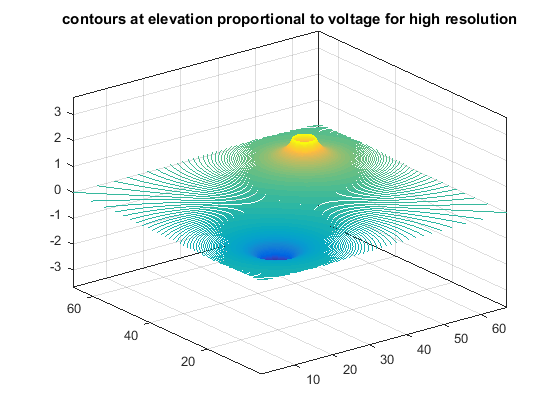
Matlab code to plot field for 2 point charges
Contents
% This matlab code is used to plot field for 2 point charges,
%minhanhnguyen@q.com
% Clear the screen
clc;
clear all;
% close all windows
close all;
input info.
Dimensionsdimension=1; d=dimension; % Charge Value charge =1; q=charge; % Creates the array of points for plotting v [x,y]=meshgrid([-d:d/33:d],[-d:d/33:d]); % Evaluate v using Coulombs Law v=-q./(4.*pi.*sqrt((x+d./2).^2+(y+d./2).^2))+q./(4.*pi.*sqrt((x-d./2).^2+(y-d./2).^2));
Plot result of equipotential contours at high resolution and countours
figure (1);
contour(v,[-1:.005:1]);
title('equipotential contours at high resolution');

%plot contours at an elevation proportional to voltage
figure;
contour3(v,[-1:.005:1]);
title('contours at elevation proportional to voltage for high resolution');

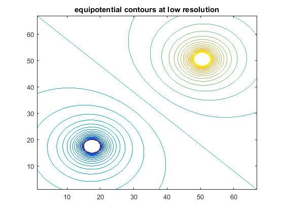
plot equipotential contours at lower resolution to see individual contours easier
figure (2);
contour(v,[-1:.05:1]);
title('equipotential contours at low resolution');

%%plot contours at an elevation proportional to voltage
figure;
contour3(v,[-1:.05:1]);
title('contours at elevation proportional to voltage');

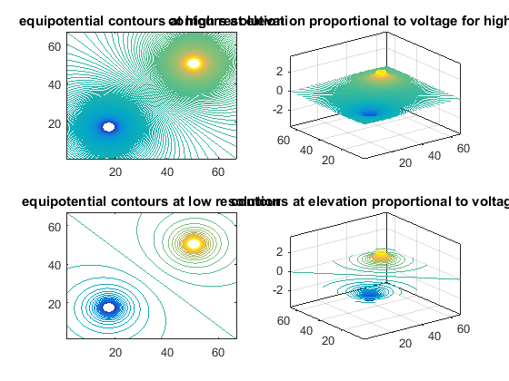
plots all four graph on the same page for comparison
figure (3);
subplot(2,2,1);contour(v,[-1:.005:1]);
title('equipotential contours at high resolution');
subplot(2,2,2);contour3(v,[-1:.005:1]);
title('contours at elevation proportional to voltage for high resolution');
subplot(2,2,3);contour(v,[-1:.05:1]);
title('equipotential contours at low resolution');
subplot(2,2,4);contour3(v,[-1:.05:1]);
title('contours at elevation proportional to voltage');
Published with MATLAB® R2015a
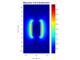
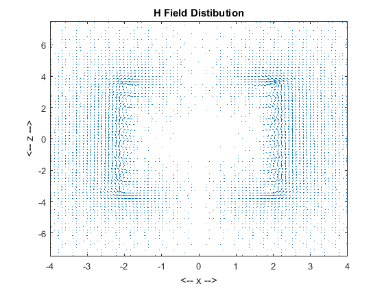
Matlab code to calculate Magnetic Flux of solenoid
Contents
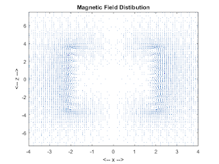
% Magnetic Flux distribution using Finite Element Method...
% of a Solenoid Vertically placed on XY plane..
% Field distribution is calculated on XZ plane @ origin (Y=0)..
% We will use Biot-Savart Law for this...
% Refer - http://en.wikipedia.org/wiki/Biot-Savart_law...
% minhanhnguyen@q.com
Contents
% Magnetic Flux distribution using Finite Element Method...
% of a Solenoid Vertically placed on XY plane..
% Field distribution is calculated on XZ plane @ origin (Y=0)..
% We will use Biot-Savart Law for this...
% Refer - http://en.wikipedia.org/wiki/Biot-Savart_law...
% minhanhnguyen@q.com
Clear the screen
clear all
clc
% close all windows
close all;
information of coil
global u0
u0=4*pi*1e-7;
d = 2; % Radius of the Loop.. (2cm = 20 mm)
m = -1; % Direction of current through the Loop... 1(ANTI-CLOCK), -1(CLOCK)
N = 30; % Number sections/elements in the conductor...
T = 10; % Number of Turns in the Solenoid..
g = 0.75; % Gap between Turns.. (mm)
dl = 2*pi*d/N; % Length of each element..
% XYZ Coordinates/Location of each element from the origin(0,0,0), Center of the Loop is taken as origin..
dtht = 360/N; % Loop elements divided w.r.to degrees..
tht = (0+dtht/2): dtht : (360-dtht/2); % Angle of each element w.r.to origin..
xC = d.*cosd(tht).*ones(1,N); % X coordinate...
yC = d.*sind(tht).*ones(1,N); % Y coordinate...
% zC will change for each turn, -Z to +Z, and will be varied during iteration...
zC = ones(1,N);
h = -(g/2)*(T-1) : g : (g/2)*(T-1);
% Length(Projection) & Direction of each current element in Vector form..
Lx = dl.*cosd(90+tht); % Length of each element on X axis..
Ly = dl.*sind(90+tht); % Length of each element on Y axis..
Lz = zeros(1,N); % Length of each element is zero on Z axis..
% Points/Locations in space (here XZ plane) where B is to be computed..
NP = 125; % Detector points..
xPmax = 3*d; % Dimensions of detector space.., arbitrary..
zPmax = 1.5*(T*g);
xP = linspace(-xPmax,xPmax,NP); % Divide space with NP points..
zP = linspace(-zPmax,zPmax,NP);
[xxP zzP] = meshgrid(xP,zP); % Creating the Mesh..
% Initialize B..
Bx = zeros(NP,NP);
By = zeros(NP,NP);
Bz = zeros(NP,NP);
% Computation of Magnetic Field (B) using Superposition principle..
% Compute B at each detector points due to each small cond elements & integrate them..
for p = 1:T
for q = 1:N
rx = xxP - xC(q); % Displacement Vector along X direction from Conductor..
ry = yC(q); % No detector points on Y direction..
rz = zzP - h(p)*zC(q); % zC Vertical location changes per Turn..
r = sqrt(rx.^2+ry.^2+rz.^2); % Displacement Magnitude for an element on the conductor..
r3 = r.^3;
Bx = Bx + m*Ly(q).*rz./r3; % m - direction of current element..
By = By - m*Lx(q).*rz./r3;
Bz = Bz + m*Lx(q).*ry./r3 - m*Ly(q).*rx./r3;
end
end
B = sqrt(Bx.^2 + By.^2 + Bz.^2); % Magnitude of B..
B = B/max(max(B)); % Normalizing...
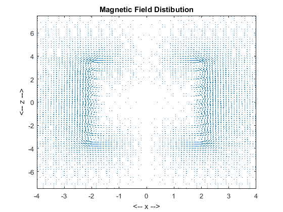
% Plotting...
test
figure(1);
pcolor(xxP,zzP,B);
colormap(jet);
shading interp;
axis equal;
axis([-xPmax xPmax -zPmax zPmax]);
xlabel('<-- x -->');ylabel('<-- z -->');
title('Magnetic Field Distibution');
colorbar;
figure(2);
surf(xxP,zzP,B,'FaceColor','interp',...
'EdgeColor','none',...
'FaceLighting','phong');
daspect([1 1 1]);
axis tight;
view(-10,30);
camlight right;
colormap(jet);
grid off;
axis off;
colorbar;
title('Magnetic Field Distibution');
figure(3);
quiver(xxP,zzP,Bx,Bz);
colormap(lines);
axis([-2*d 2*d -T*g T*g]);
title('Magnetic Field Distibution');
xlabel('<-- x -->');ylabel('<-- z -->');
zoom on;
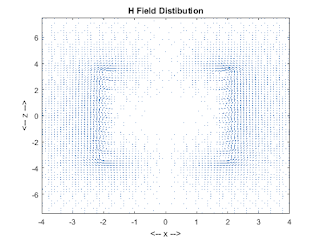
% Computation of (H)Field using Superposition principle..
% Compute H at each detector points due to each small cond elements & integrate them..
for p = 1:T
for q = 1:N
rx = xxP - xC(q); % Displacement Vector along X direction from Conductor..
ry = yC(q); % No detector points on Y direction..
rz = zzP - h(p)*zC(q); % zC Vertical location changes per Turn..
r = sqrt(rx.^2+ry.^2+rz.^2); % Displacement Magnitude for an element on the conductor..
r3 = r.^3;
Hx = (Bx + m*Ly(q).*rz./r3)*u0; % m - direction of current element..
Hy = (By - m*Lx(q).*rz./r3)*u0;
Hz = (Bz + m*Lx(q).*ry./r3 - m*Ly(q).*rx./r3)*u0;
end
end
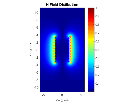
H= sqrt(Hx.^2 + Hy.^2 + Hz.^2); % Magnitude of H..
H = H/max(max(H)); % Normalizing...

test
figure(1);
pcolor(xxP,zzP,H);
colormap(jet);
shading interp;
axis equal;
axis([-xPmax xPmax -zPmax zPmax]);
xlabel('<-- x -->');ylabel('<-- z -->');
title('H Field Distibution');
colorbar;
figure(2);
surf(xxP,zzP,H,'FaceColor','interp',...
'EdgeColor','none',...
'FaceLighting','phong');
daspect([1 1 1]);
axis tight;
view(-10,30);
camlight right;
colormap(jet);
grid off;
axis off;
colorbar;
title('H Field Distibution');
figure(3);
quiver(xxP,zzP,Hx,Hz);
colormap(lines);
axis([-2*d 2*d -T*g T*g]);
title('H Field Distibution');
xlabel('<-- x -->');ylabel('<-- z -->');
zoom on;


Published with MATLAB® R2015a


example of plot and find and mark maximum and minimum values on a plot using Matlab
Contents
example of plot and find and mark maximum and minimum values on a plot
Author: minhanhnguyen@q.comclose
close all; % Clear all windows
clear all; % Clear all variables
clc; % Clear console
generate a simple plot
x = linspace(-3,3);
y = (x/5-x.^3).*exp(-2*x.^2);
plot(x,y)

find the mimimum value
indexmin = find(min(y) == y);
xmin = x(indexmin);
ymin = y(indexmin);

strmin = ['Minimum = ',num2str(ymin)];
text(xmin,ymin,strmin,'HorizontalAlignment','left');

find the max value
indexmax = find(max(y) == y); xmax = x(indexmax); ymax = y(indexmax); strmax = ['Maximum = ',num2str(ymax)]; text(xmax,ymax,strmax,'HorizontalAlignment','right');

example to display MRI image and data
close
close all; % Clear all windows
clear all; % Clear all variables
clc; % Clear console

% load the data and transform the data array from 4-D to 3-D
% The MRI data, D, is stored as a 128-by-128-by-1-by-27 array.
% Use the squeeze command to remove  4-D to 3-D.
% The result is a 128-by-128-by-27 array
load mri
D = squeeze(D);
display one of the MRI images
figure
colormap(map)
image_num = 10;
image(D(:,:,image_num))
axis image
x = xlim;
y = ylim;


2-D Contour Slice
contour plot uses the jet colormaptwodc = brighten(jet(length(map)),-.5);
figure;
colormap(twodc);
contourslice(D,[],[],image_num)
axis ij
xlim(x)
ylim(y)
daspect([1,1,1])

%%3-D Contour Slices
figure
colormap(twodc)
contourslice(D,[],[],[1,12,19,27],10);
view(3);
axis tight

%%Isosurface to the MRI Data
figure
colormap(map)
Ds = smooth3(D);
hiso = patch(isosurface(Ds,5),...
   'FaceColor',[1,.75,.65],...
   'EdgeColor','none');
   isonormals(Ds,hiso);


Isocaps Show Cut-Away Surface
 hcap = patch(isocaps(D,5),...
   'FaceColor','interp',...
   'EdgeColor','none');

Defining the View
%Define the view and set the aspect ratio (view, axis, daspect).


view(75,30)
axis tight
daspect([1,1,.4])
lightangle(75,30);

lighting gouraud
hcap.AmbientStrength = 0.5;
hiso.SpecularColorReflectance = 0;
hiso.SpecularExponent = 60;

figure;

close;


Slices 3-Dimensional MRI Data
load mri;%Load the MRI data
figure; montage(D,map) %view the 27 horizontal slices as a montage.
title('Horizontal Slices');

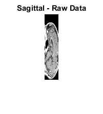
M1 = D(:,64,:,:); size(M1);
M2 = reshape(M1,[128 27]); size(M2)
figure; imshow(M2,map);
title('Sagittal - Raw Data');
T0 = maketform('affine',[0 -2.5; 1 0; 0 0]);

R2 = makeresampler({'cubic','nearest'},'fill');
M3 = imtransform(M2,T0,R2);
figure; imshow(M3,map);
title('Sagittal - IMTRANSFORM');

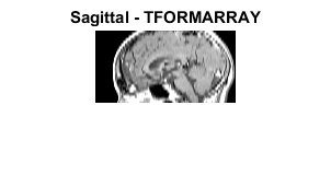
T1 = maketform('affine',[-2.5 0; 0 1; 68.5 0]);
inverseFcn = @(X,t) [X repmat(t.tdata,[size(X,1) 1])];
T2 = maketform('custom',3,2,[],inverseFcn,64);
Tc = maketform('composite',T1,T2);

R3 = makeresampler({'cubic','nearest','nearest'},'fill');

M4 = tformarray(D,Tc,R3,[4 1 2],[1 2],[66 128],[],0);
figure; imshow(M4,map);
title('Sagittal - TFORMARRAY');
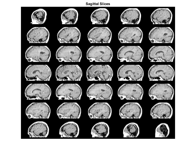
T3 = maketform('affine',[-2.5 0 0; 0 1 0; 0 0 0.5; 68.5 0 -14]); S = tformarray(D,T3,R3,[4 1 2],[1 2 4],[66 128 35],[],0); S2 = padarray(S,[6 0 0 0],0,'both'); figure, montage(S2,map) title('Sagittal Slices');M1 = D(:,64,:,:); size(M1) M2 = reshape(M1,[128 27]); size(M2) figure, imshow(M2,map); title('Sagittal - Raw Data');
R2 = makeresampler({'cubic','nearest'},'fill');
M3 = imtransform(M2,T0,R2);
figure, imshow(M3,map);
title('Sagittal - IMTRANSFORM')


T1 = maketform('affine',[-2.5 0; 0 1; 68.5 0]);
inverseFcn = @(X,t) [X repmat(t.tdata,[size(X,1) 1])];
T2 = maketform('custom',3,2,[],inverseFcn,64);
Tc = maketform('composite',T1,T2);


M4 = tformarray(D,Tc,R3,[4 1 2],[1 2],[66 128],[],0);


figure, imshow(M4,map);
title('Sagittal - TFORMARRAY');


T3 = maketform('affine',[-2.5 0 0; 0 1 0; 0 0 0.5; 68.5 0 -14]);


S = tformarray(D,T3,R3,[4 1 2],[1 2 4],[66 128 35],[],0);


S2 = padarray(S,[6 0 0 0],0,'both');
figure, montage(S2,map)
title('Sagittal Slices');


T4 = maketform('affine',[-2.5 0 0; 0 1 0; 0 0 -0.5; 68.5 0 61]);

C = tformarray(D,T4,R3,[4 2 1],[1 2 4],[66 128 45],[],0);
C2 = padarray(C,[6 0 0 0],0,'both');
figure, montage(C2,map)
title('Coronal Slices');

ans =

   128    27


ans =

   128     1     1    27


ans =

   128    27


Subscribe to:
Posts (Atom)