Purpose
The
purpose of this analysis is to determine if the method of comparing two image
files can be used for
detecting of human errors for channel-not-loaded-correctly issue. There
are many algorithms which can be used to compare two image files. These algorithms are: edge detection, Short
Time Fourier Transform (STFT), wavelet, and histogram. In this project, histogram algorithm is used
to compare two image files.
Why use Histogram
Histogram is a way of visualizing
the largest intensities of an image. It is used to depict problems which
originate during image acquisition such as exposure, contrast, dynamic range. The contrast of a
grayscale image shows how easily objects in the image can be distinguished. The
dynamic range is the number of distinct pixel value in an image. It is used to show image statistics in an easily interpreted visual
format. It
is also a
graph showing the number of pixels in an image at each different intensity
value found in that image. The
histogram of a digital image is a distribution of its discrete intensity levels
in the range [0, L-1]. The number of possible intensity values depends on the
numerical type encoding the image.
For example,
a grayscale image encoded with n=8
bits, it will has an
array of size L=28=256. The number of
possible intensity values go from 0 representing black to L-1=255 representing
white. Since there are 256 different possible
intensities, the histogram will graphically display 256 numbers showing the
distribution of pixels amongst those greyscale values. When
represented as a plot, the x-axis is the intensity value from 0 to 255, and the
y-axis is the number of pixels with that intensity value. The y-axis varies depending on the number of
the pixels in the image and how their intensities are distributed as shown in
figure 2. An image has only one histogram,
but many images may have the same histogram.
Histograms
have many uses. One of the more common is to
determine if the overall intensity in the image is high enough for this
inspection task. Histogram is used to determine whether an image contains
distinct regions of certain grayscale values.
If
the image has poor dynamic range, then the histogram confirms what one can see
by visual inspection. It provides a general description of
the appearance of an image and helps identify various components such as the
background, objects, and noise.
How Histogram Works
The
operation is very simple. The image is scanned in a single pass and a running
count of the number of pixels found at each intensity value is kept. This is
then used to construct a suitable histogram.
The histogram of an 8-bit image, for example can be thought of as a
table with 256 entries, or ‘bins’, indexed from 0 to 255. In bin 0 we record
the number of times a gray level of 0 occurs; in bin 1 we record the number of
times a grey level of 1 occurs, and so on, up to bin 255.
Techniques for comparing two image files
Step1: read images
Read
two grayscale images into the workspace.
Step 2: Resize images
To
make the image comparison easier, resize the images to have the same width.
Step 3: Find matching features
between images
Step 4: Display error message on the
computer monitor screen, if images are not matched.
Flow chart for comparing two image files

Figure1. Flow chart for comparing two image files
Image test in simulation
mode
The
following steps are a procedure to test the image in simulation mode.
1.
Make
sure image files are loaded into the workspace without any issues.
2.
Make
sure a correct file is loaded
3.
Plot
histogram of the image
4.
Verify
that the histogram value is correct.
5.
Positive
test: load two image files which have 2 different images and verify that the
test results show the difference.
6.
Negative
test: load two image files which have 2 similar images and verify that the test
results show the same thing or match.
Software
Matlab R2015b
Labview
2014
Summary of
results
The following figure illustrates the
difference between the displays of the histogram of the same image in a linear
and the results of the techniques and flow chart for comparing two image files
above.

Figure2.
Matlab results for comparing two images which are identical.

Figure3.
Matlab results for comparing two images which are not identical. The object
being viewed is light in color and it is placed on a dark background, and so
the histogram exhibits a good bi-modal distribution. One peak represents the
object pixels, other represents the background.

Figure4.
Matlab results for comparing two images which are not identical. The object
being viewed is dark in color and it is placed on a light background, and so
the histogram exhibits a good bi-modal distribution. One peak represents the
object pixels, one represents the background. The peak represents of back ground is at the
highest intensity value, X = 241.

Figure5. Matlab results for comparing two hex pin
images which are identical. The resulting of histograms above showed a large
spike at 250 intensity value which results in the rest of the histogram being
scaled up to 256.

Figure6.
Matlab results for comparing two hex pin images which are not identical
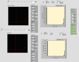
Figure7. Labview results for comparing two image
files which are identical

Figure8. Labview results for comparing two image
files which are not identical
These results showed that the method of comparing
two image files can be used for
detecting of human errors for channel-not-loaded-correctly issue. A histogram is the frequency distribution of the gray levels
with the number of pure black values displayed on the left and number of pure
white values on the right.
Matlab Code for comparing two image
files.
%% Matlab Code:
% Author: Minh Anh Nguyen
(minhanhnguyen@q.com)
%This function will perform
the followign tasks:
%1. read in two
".png" file, display both images on the computer screen.
%2. histogram of the images
% 3. compare both image
files.
% 4. display a message on
the computer screen if both image are not the
% same.
function [imagefunction]
= imagefunction( file1, file2 );
% clear all; % Erase all
existing variables.
close all; % Close
all figures (except those of imtool.)
clc;% Clear
the command window.
imtool close all; % Close
all imtool figures.
workspace; % Make
sure the workspace panel is showing.
fontSize = 20;
%%%%%%%%%%%%%
% %% team: edit your file
here
% %%% set the path
% folder =
'I:\F2015_486A\image';
% %reading images as array
to variable 'a' & 'b'.
image1 = imread( file1 );
image2= imread( file2 );
%
% %reading images as array
to variable 'a' & 'b'.
% image1 =
imread('Loaded-Mid Channel.PNG');
% image2= imread('Gross
Misloaded-Mid Channel.PNG');
%
% %% info
imfinfo( file1 )
imfinfo( file2)
%%%%%%%%%%%%%%%%%%%%%%%%%%%%%%%%%%%%%%%%%%%%%%%%
% do not edit anything
below here!!!!
%%%%%%%%%%%%%%%%%%%%%%%%%%%%%%%%%%%%%%%%%%%%%%%%%%%%%%%%%%%%%%%%%%%%%%
a = image1;
b = image2;
%% size
a1= size(a);
b1= size (b);
figure;
[rows columns numberOfColorBands]
= size(a);
subplot(2, 2, 1); imshow(a, []);
title('Reference
image', 'Fontsize', fontSize);
set(gcf, 'Position', get(0,'Screensize')); % Maximize
figure.
redPlane = a(:, :, 1);
greenPlane = a(:, :, 2);
bluePlane = a(:, :, 3);
[rows columns numberOfColorBands]
= size(b);
subplot(2, 2, 3); imshow(b, []);
title('Image2', 'Fontsize', fontSize);
set(gcf, 'Position', get(0,'Screensize')); % Maximize
figure.
redPlane1 = b(:, :, 1);
greenPlane1 = b(:, :, 2);
bluePlane1 = b(:, :, 3);
% Let's get its histograms.
[pixelCountR grayLevelsR] =
imhist(redPlane);
subplot(2, 2, 2); %plot(pixelCountR,
'r');
stem(grayLevelsR,pixelCountR, 'r');
title('Histogram of
Reference image', 'Fontsize', fontSize);
xlabel('Intensity
values','Fontsize', fontSize);
ylabel('Number of
pixels', 'Fontsize', fontSize);
xlim([0 grayLevelsR(end)]); % Scale x
axis manually.
[pixelCountR1 grayLevelsR1] =
imhist(redPlane1);
subplot(2, 2, 4);
%plot(pixelCountR1, 'r');
stem(grayLevelsR1,pixelCountR1);
title('Histogram of
Image2', 'Fontsize', fontSize);
xlabel('Intensity
values','Fontsize', fontSize);
ylabel('Number of
pixels','Fontsize', fontSize);
xlim([0 grayLevelsR1(end)]); % Scale x
axis manually.
%check image for different
different = a1- b1
if different==0
disp('The images are same')%output
display
else
disp('the images are not same')
msgbox('Test error. Please check your
setting', 'Error')
end;
Labview Code for comparing two image
files.

No comments:
Post a Comment